原文作者: Will Wilson
原文链接: https://antithesis.com/blog/2026/skiptrees/
为防遗失,转载一份。
A while back, I joined Phil Eaton’s book club on The Art of Multiprocessor Programming, and the topic of skiplists came up.
For most of my career, skiplists had always seemed like a niche data structure, with a rabid cult following but not a whole ton of applicability to my life. Then six or so years ago, we encountered a problem at Antithesis that seemed intractable until it turned out that a generalization of skiplists was exactly what we needed.
Before I tell you about that, though, let me explain what skiplists are (feel free to skip ahead if you already know them well).
What are skiplists?
A skiplist is a randomized data structure that’s basically a drop-in replacement for a binary search tree with the same interface and the same asymptotic complexity on each of its operations. Some people like them because you can produce relatively simple and understandable lock-free concurrent implementations, and others like them as a matter of taste, or because they enjoy listening to bands that you’ve totally never heard of.
In implementation terms, you can think of them roughly as linked lists plus “express lanes”:
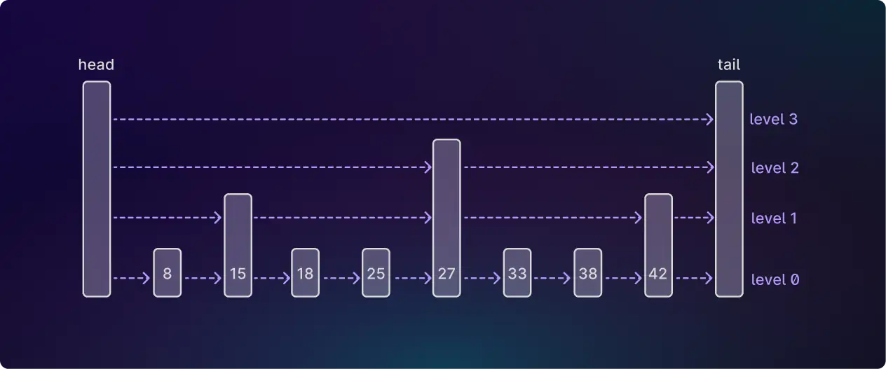
You start with a basic linked list, and then add a hierarchy of linked lists with progressively fewer nodes in them. In the example above, the nodes in the higher-level lists are chosen probabilistically, with each node having a 50% chance of being promoted to the next level. For (much) more on skiplists, see The Ubiquitous Skiplist(https://arxiv.org/pdf/2403.04582).
This helps with search, because you can use the higher-level lists to skip more quickly to the node you want:
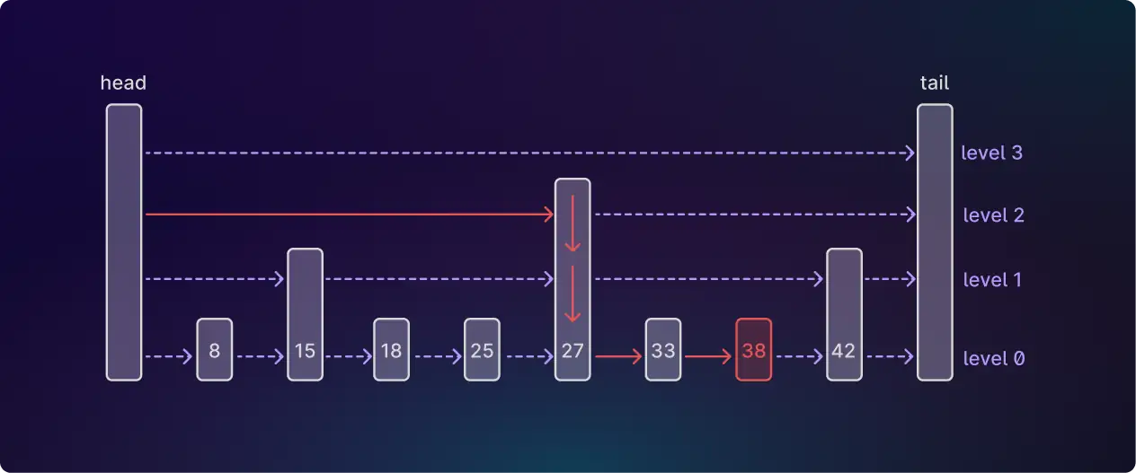
Here we’ve found the node with an ID of 38 by starting at the top level and working downwards. At each level we advance until the next node would have an ID that’s too high, then jump down a level.
In a regular linked list of n nodes, finding a node would take O(n) time, because you’re walking through the nodes one by one. Skiplists let you jump levels, with each level halving the number of nodes you need to check, so you end up finding the node in O(log n) time.
This is all very nice, but after reading about this data structure I literally never thought about it again, until one day we encountered the following problem at Antithesis…
The problem
Antithesis runs customers’ software many times to look for bugs. Each time, our fuzzer injects different faults and tells your testing code to make different random decisions. Over many runs, these choices create a branching tree of timelines: each path from root to leaf represents one sequence of choices the fuzzer made and what happened as a result.
There were a lot of queries that we wanted to do which basically amounted to fold operations up or down this tree. For example, given a particular log message, what’s the unique history of events that led to it? (Walk up the parent pointers from that node to the root.)
The trouble was that the amount of data output by the software we were testing was so huge, we had to throw it all into an analytic database, and at the time we were using Google BigQuery. Analytic databases are optimized for scanning massive amounts of data in parallel to compute aggregate results. The tradeoff is that they’re slow at point lookups, where you fetch a specific row by its ID.
This matters, because the natural way to represent a tree in a database is with parent pointers — each node is a row in the table, with a parent_id column pointing to its parent. To answer a question like “show me the history leading to this log message”, you’d need to walk up the tree one node at a time: look up the node, get its parent ID, look up the parent node, and so on. Each step is a point lookup. In an OLTP database designed for point lookups, that’s fine. I mean, not actually, but it's less bad. But in BigQuery, basically every operation results in a full table scan, which means even the most basic queries would end up doing O(depth) reads over your entire data set. Yikes!
One alternative would have been to split the data: store just the tree structure (the parent pointers) in a database that’s good at point lookups, and keep the bulk data in BigQuery. But this approach would have created other problems. Every insert would need to write to both systems, and since we want to analyze the data online (while new writes are streaming in) keeping the two databases consistent would require something like two-phase commit (2PC). I prefer not to invent new 2PC problems where I don’t need them. And anyway, at the time BigQuery had very loose consistency semantics, so it’s not even clear that keeping the two systems in sync would have been possible.
Skiplists to the rescue! Or rather, a weird thing we invented called a “skiptree”…
What’s a skiptree?
Well, it’s like a skiplist, but it’s a tree.
More helpfully, here’s an example:
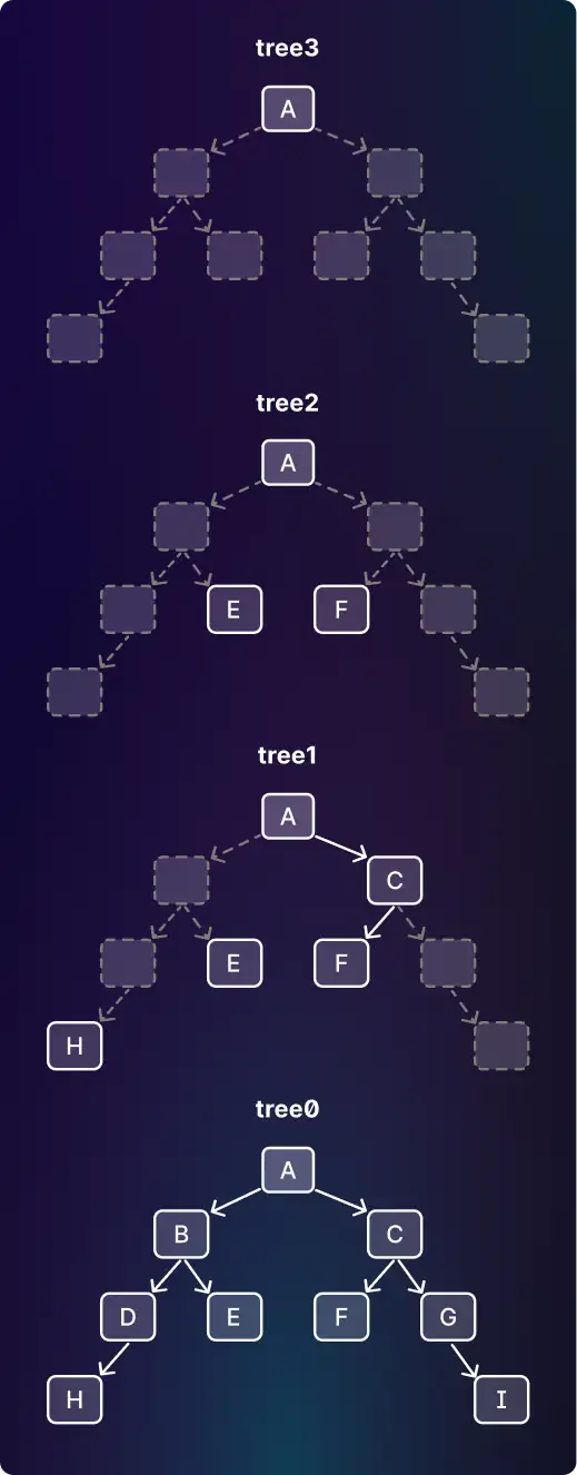
You have a level-0 tree, and then a hierarchy of trees above it. Each tree has roughly 50% of the nodes of the level below (the removed nodes are shown with grey dotted lines on the diagram).
If you pick any path from the root to a leaf, the nodes along that path — together with their appearances in the higher-level trees — form a skiplist. So a skiptree is really just a bunch of skiplists sharing structure, one for every root-to-leaf path in the tree.
To store the skiptree, you create a SQL table for each level: tree0, tree1, and so on. Each table has a row for every node in that tree. Instead of having a single parent_id column, it has a column for the closest ancestor node in the tree above (we’ll call that next_level_ancestor) and another column (call it ancestors_between) with a list of all nodes between the current node and the next-level ancestor.
For the diagram above, tree0 would look like this:
| id | next_level_ancestor | ancestors_between |
|---|---|---|
| A | null | [] |
| B | A | [] |
| C | A | [] |
| D | A | [B] |
| E | A | [B] |
| F | C | [] |
| G | C | [] |
| H | A | [B,D] |
| I | C | [G] |
As an example, take the row for node H. Node H’s parent is D, which is not in tree1. D’s parent B is also not in tree1, but B’s parent A is, so next_level_ancestor is A. Then ancestors_between stores B and D.
The higher-level tables work the same way:
tree1:
| id | next_level_ancestor | ancestors_between |
|---|---|---|
| A | null | [] |
| C | A | [] |
| E | A | [B] |
| F | C | [] |
| H | A | [B,D] |
tree2:
| id | next_level_ancestor | ancestors_between |
|---|---|---|
| A | null | [] |
| E | A | [B] |
| F | A | [C] |
tree3:
| id | next_level_ancestor | ancestors_between |
|---|---|---|
| A | null | [] |
You can use these tables to find the ancestors of a node by chaining together JOINs, working your way up the tables.
这里构建表的步骤是:
1. 从 level 0 (即 tree0)开始构造,每个 level 表构造完成后再构造下一级的表。所有层级的表都包含根节点,“最深层级”的表仅包含根节点。tree0 表的行包含了全部的节点,每“增加一级”的表中,除去根节点以外的行数为“上一级”表的一半。
2. 首先构造 tree0 表。从根节点(它的 next_level_ancestor 固定为 null ,ancestors_between 固定为空数组)开始,广度优先遍历所有节点,每遍历到一个节点,将其作为一个新行插入到 tree0 表中,id 列保持这个插入的顺序。每个被遍历到的节点,如果它的父节点为根节点,则它的 next_level_ancestor 的值为根节点,ancestors_between 的值为空数组;如果它的父节点不是根节点,则以 50% 的概率按以下两种情况之一来取 next_level_ancestor 和 ancestors_between 列的值:
2-1. 取它的父节点的 id 为自己的的 next_level_ancestor , ancestors_between 的值为空数组。
2-2. 取它的父节点在 tree0 表中的行的 next_level_ancestor 及 ancestors_between 的值为自己相应列的值,再将父节点的id加入到 ancestors_between 数组的尾部。
3. 接着构造 tree1 表。从 tree0 表中以 50% 的概率取除去根节点外的一半节点,加上根节点,作为 tree1 表中的行。检查 tree1 表中的每一行/节点的 next_level_ancestor 列的值,如果这个值对应的节点 x 不在 tree1 表中,则从低一个层级的表(对 tree1 表来说,就是 tree0 表)中,取 id=x 的行的 next_level_ancestor 及 ancestors_between 的值为自己相应列的值,再将 x 加入到 ancestors_between 数组的尾部。更新后的 next_level_ancestor 的值 y 如果还是不在 tree1 表中,则继续从 tree0 表中取 y 的 next_level_ancestor 作为这一行 next_level_ancestor 新的值,y 再加入到 ancestors_between 数组的尾部 ... ... 重复这个过程,直到 next_level_ancestor 最新的值代表的节点,是 tree1 表中已存在的节点。
4. 类似上面的步骤,依次构造 tree2 、tree3 ... treeN 表,直到“最高层级”的表中只有根节点一个节点。
For example, to find all ancestors of node I, start at table0. The next_level_ancestor column tells you to JOIN on node C in table1, collecting node G from the ancestors_between column on the way. Then in table1 you find that the next_level_ancestor is node A, with no other nodes to collect on the way. Node A is the root of the tree so you’re now done: the total list of ancestors is [G, C, A]. In a deeper tree you’d keep going by looking in tree2, tree3 and so on.
Hey! Now we can find ancestors with a single non-recursive SQL query with a fixed number of JOINs. We just had to do… 40 or so JOIN. The number of skip levels was precisely chosen to generate a number of joins just under the BigQuery planner's hard-coded limit.
Best of all, at the time BigQuery’s pricing charged you for the amount of data scanned, rather than for compute, and the geometric distribution of table sizes meant that each of these queries only cost twice a normal table scan. I'm sure it cost Google a whole lot more.
Of course, there were disadvantages, like the SQL itself. The textual size of these queries was often measured in the kilobytes. But what do I look like, a caveman? We didn’t write the SQL. We wrote a compiler in JavaScript that generated it. And that is how most test properties in Antithesis were evaluated for the first six years of the company, until we finally wrote our own analytic database that could do efficient tree-shaped queries. Migrating from BigQuery to Pangolin (our in-house tree database) was what enabled us to launch our new pre-observability(https://antithesis.com/blog/2025/logs_explorer/) feature last year.
Skiplists, skiptrees, skipgraphs…
Later I discovered that a skiptree is closely related to a real data structure called a skip graph, a distributed data structure based on skiplists. Which just goes to show that there is nothing new under the sun. Whatever crazy idea you have, there’s a good chance some other crazy person has already done it. Moral of the story: you never know when an exotic data structure will save you a lot of time and money.
Also, while Andy Pavlo is correct that a well-written tree will always trounce a skiplist, the great thing about skiplists is that a totally naive implementation has adequate performance. That comes in handy when you’re writing them in, say, SQL.
Thank you to Phil Eaton for suggesting that we write this up.

Comments